0%

用SVM(支持向量机)处理分类问题

支持向量机(SVM)是一系列可用于分类、回归和异常值检测的有监督学习方法。本文讨论 SVM 在分类问题上的应用。

SVM 的优点包括:

* 在高维空间中行之有效。
* 当维数大于样本数时仍然可用。
* 在决策函数中只使用训练点的一个子集(称为支持向量),大大节省了内存开销。
* 用途广泛:决策函数中可以使用不同的核函数。提供了一种通用的核,但是也可以指定自定义的核

劣势在于:

* 如果特征数量远大于样本数量,则表现会比较差。
* SVM不直接提供概率估计。这个值通过五折交叉验证计算,代价比较高

SVM原理

处理分类问题,一个直接的思路是构建一条直线/超平面,将样本按照类别标签进行划分,然后用这条直线/超平面进行预测。
这条超平面最好能使得点到决策边界的距离最大化[^1]。

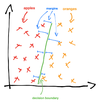
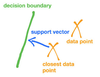
支持向量(support vectors),就是点到决策边界的最小间隔时的向量(由点出发垂直指向边界)。

如果样本线性不可分,就通过某种函数变换,使其变得线性可分,然后在求解直线/超平面。
这个函数变换,在SVM中称为核函数(kernel function)

最后,有可能会有个别的点无法正确分类,有时候要允许这种情况的发生。此时可以增加一个松弛变量/损失函数来适应这种情况。
在机器学习中,这种情况称之为正则,通常使用正则化参数来处理:

在我们的损失函数中添加一项:C(惩罚因子)。
对训练集的每一个数据点,给出特定的惩罚因子 c,c 越大表示偏离决策边界的损失越大。

更深入的理解,强烈推荐阅读资料[^2]。

scikit-learn对SVM的支持

Scikit-learn中的支持向量机同时支持密集样本向量( numpy.ndarray 和可通过 numpy.asarray 转化的数据类型)和
稀疏样本向量(任何 scipy.sparse 对象)。但是如果想用SVM对稀疏数据进行预测,则必须先在这些数据上拟合。
为了优化性能,应该使用C阶(C-Ordered) numpy.ndarray (密集的)或 scipy.sparse.csr_matrix (稀疏的),
并指定 dtype=float64 。

在分类问题上,可以使用 SVC , NuSVC 和 LinearSVC 这三个类。

SVC 和 NuSVC 两种方法类似,但是接受的参数有细微不同,而且底层的数学原理不一样。

LinearSVC 中,核函数被设定为线性的(线性核)。

scikit-learn的 SVM 分析鸢尾花数据集

import pandas as pd
import warnings 
# 用来忽略seaborn绘图库产生的warnings
warnings.filterwarnings("ignore")
import seaborn as sns
import matplotlib.pyplot as plt
sns.set(style="white", color_codes=True)
%pylab inline
Populating the interactive namespace from numpy and matplotlib

数据概览

from sklearn.datasets import load_iris
iris = load_iris()
df = pd.DataFrame(iris.data,columns=['sepal_length','sepal_width','petal_length','petal_width'])
df['target']=pd.Series(iris.target)
df.head()
Out[2]:
sepal_length sepal_width petal_length petal_width target
0 5.1 3.5 1.4 0.2 0
1 4.9 3.0 1.4 0.2 0
2 4.7 3.2 1.3 0.2 0
3 4.6 3.1 1.5 0.2 0
4 5.0 3.6 1.4 0.2 0
sns.FacetGrid(df, hue="target", size=5).map(plt.scatter, "sepal_length", "sepal_width").add_legend()
sns.FacetGrid(df, hue="target", size=5).map(plt.scatter, "petal_length", "petal_width").add_legend()
Out[3]:
<seaborn.axisgrid.FacetGrid at 0x10e0c3cc0>

模型训练

# 拆分数据
from sklearn.cross_validation import train_test_split
x_train, x_test, y_train, y_test = train_test_split(df[['sepal_length','sepal_width']], df['target'], random_state=1)

# 训练
from sklearn import svm
model = svm.SVC()
model.fit(x_train,y_train) 
/usr/local/Cellar/python3/3.6.2/Frameworks/Python.framework/Versions/3.6/lib/python3.6/site-packages/sklearn/cross_validation.py:41: DeprecationWarning: This module was deprecated in version 0.18 in favor of the model_selection module into which all the refactored classes and functions are moved. Also note that the interface of the new CV iterators are different from that of this module. This module will be removed in 0.20.
  "This module will be removed in 0.20.", DeprecationWarning)
Out[5]:
SVC(C=1.0, cache_size=200, class_weight=None, coef0=0.0,
  decision_function_shape='ovr', degree=3, gamma='auto', kernel='rbf',
  max_iter=-1, probability=False, random_state=None, shrinking=True,
  tol=0.001, verbose=False)
# 训练结果

# get support vectors
print(model.support_vectors_)

# get indices of support vectors
print(model.support_)

# get number of support vectors for each class
print(model.n_support_)
[[ 5.7  3.8]
 [ 4.8  3. ]
 [ 5.5  3.5]
 [ 4.8  3. ]
 [ 5.1  3.3]
 [ 5.7  4.4]
 [ 4.5  2.3]
 [ 4.9  3. ]
 [ 5.4  3.4]
 [ 5.   3. ]
 [ 6.5  2.8]
 [ 6.6  2.9]
 [ 5.2  2.7]
 [ 6.   3.4]
 [ 5.7  3. ]
 [ 6.7  3.1]
 [ 5.7  2.8]
 [ 6.   2.2]
 [ 6.4  2.9]
 [ 5.   2.3]
 [ 6.   2.7]
 [ 5.8  2.7]
 [ 6.2  2.9]
 [ 6.3  2.3]
 [ 5.6  2.9]
 [ 5.8  2.7]
 [ 6.9  3.1]
 [ 6.8  2.8]
 [ 5.9  3.2]
 [ 5.6  3. ]
 [ 5.   2. ]
 [ 4.9  2.4]
 [ 5.9  3. ]
 [ 6.1  2.9]
 [ 6.7  3.1]
 [ 5.7  2.9]
 [ 6.2  2.2]
 [ 7.   3.2]
 [ 6.1  2.8]
 [ 5.7  2.6]
 [ 6.3  2.5]
 [ 6.7  2.5]
 [ 6.   2.2]
 [ 6.3  2.9]
 [ 7.7  2.6]
 [ 7.7  3.8]
 [ 6.4  2.8]
 [ 6.2  2.8]
 [ 5.7  2.5]
 [ 6.3  2.7]
 [ 6.5  3. ]
 [ 6.1  3. ]
 [ 6.5  3.2]
 [ 6.   3. ]
 [ 6.5  3. ]
 [ 6.3  3.3]
 [ 6.4  2.7]
 [ 5.9  3. ]
 [ 6.7  3. ]
 [ 6.2  3.4]
 [ 6.3  3.4]
 [ 5.6  2.8]
 [ 5.8  2.7]
 [ 6.5  3. ]
 [ 4.9  2.5]
 [ 6.4  3.2]
 [ 5.8  2.7]
 [ 6.1  2.6]
 [ 6.3  2.8]
 [ 6.4  3.1]]
[  8  10  13  25  51  62  64  90 101 102   0   6  11  19  21  31  32  36
  37  39  47  52  55  58  61  63  66  68  76  85  88  91  93  94  96  97
  98  99 104 106 109   1   4   5   7  14  17  18  23  24  27  29  30  34
  38  40  48  49  57  59  71  72  78  80  81  83 100 103 107 108]
[10 31 29]
# 检查得分
model.score(x_test,y_test)
Out[10]:
0.81578947368421051
 

参考资料

[^1]: 感知机、逻辑回归、支持向量机- 伯克利机器学习入门教程
[^2]: 支持向量机通俗导论(理解SVM的三层境界)